


Convolutional Neural Networks (CNN) have been used succesfully on fields such as Computer Vision or Natural Language Processing, being a reliable method for image recognition tasks such as identifying faces, objects and traffic signs, apart from powering vision in robots and self driving cars.
The architecture of a typical CNN is composed of two stages. First, a series of one or more convolutional layers are used to extract and learn high-level features from the input. Then, one or more fully connected layers perform the classification task.
What is a convolution?
A convolution can be seen as a sliding window function applied to the input data. To visualize this, let's supose we have an input matrix like this:

and we want to apply the next convolution:

The process is showed in the next animation. The convolution is applied as a sliding window, which is typically called kernel or filter, over the input data. The dimmension of the output will depend on the sizes of the input and the filter. In this case, the input size is 5x5 and the filter is 3x3. If the sliding window moves 1 position at a time, the generated output will be a 3x3 matrix.

Architecture of a convolutional network
CNNs are composed of several layers of convolutions with nonlinear activation functions like ReLU or tanh applied to the results, connected to set of fully connected layers that acts as a classifier that uses the high-level features produced by the convolutional layers.
Each convolutional layer applies a specified number of convolution filters to its input. For each subregion of a specified dimmension (kernel), it performs a set of mathematical operations to generate a single value in the output feature map. This output map can be used as the input of another convolutional layer, incrementing the level of complexity and the power of the network. This way, each filter builds a feature map over the previously built by the precedent layer, transforming those features into a higher level representation. If the input is an image, it makes intuitive sense that the first layer will build edges from pixels, the second shapes from edges, the third more complex objects from shapes, and so on.
In order to decrease the level of complexity when many convolutional layers are stacked, it is common to downsample the data extracted by each layer, tipically by using algorithms such as max pooling or average pooling. These algorithms extract subregions of the feature map, apply an operation to its values (maximum, average, etc), and keep this value, discarding the original ones. Using a pooling size of 3x3, the dimmension of a feature map of 150x150 would be reduced to 50x50.
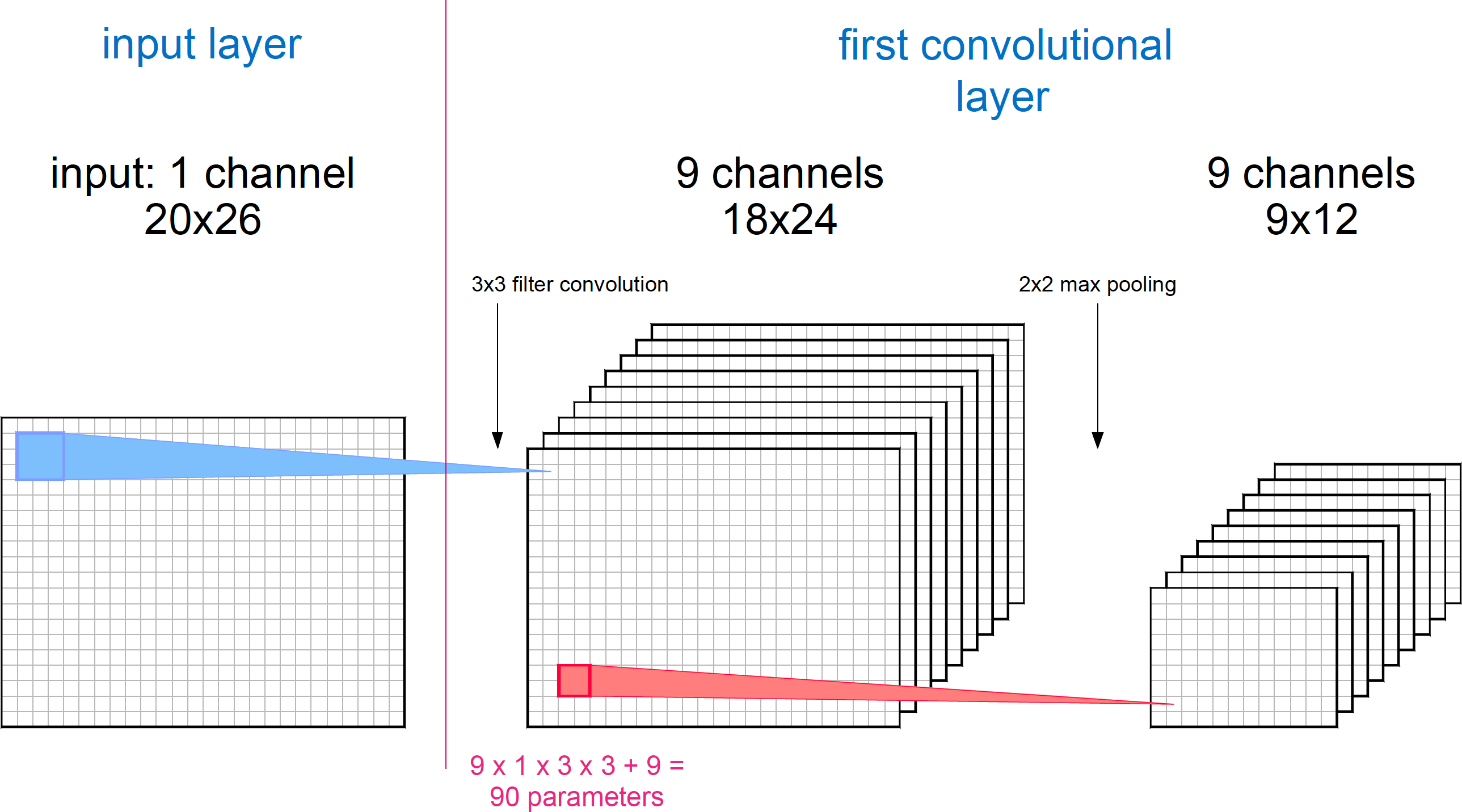
The following images describe the architecture we're going to implement. The input will be reshaped from its original shape, vectors of 520 features, to a 3D matrix of dimmensions 1x20x26. By analogy, this would represent an image of 26x20 pixels and only 1 channel (a greyscale image):

The input is connected to the first convolutional module. The dimmension of the convolutional filter will be 3x3 'pixels', and the number of filters will be 9. The downsampling stage of this layer will use a 2x2 max pooling filter. The convolutional step of the module will output nine feature maps of size 18x24, one for each filter applied. The 2x2 max pooling algorithm will downsample them to a size of 9x12.
The number of parameters that the model will have to learn during training is:
- 3x3 parameters for each filter -> 3x3x9 = 81
- 1 bias parameter for each filter -> 1x9 = 9
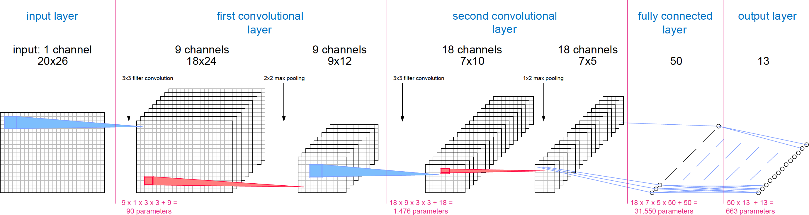
Now, the output of the first convolutional module is used as input for the second convolutional layer, thus the dimmension of the input is 9x9x12. We will apply 18 convolutional filters of size 3x3 to each input channel and a 1x2 max pooling algorithm, so the output od this stage will be of size 18x7x5.
The number of parameters of this module is:
- 3x3 parameters for each filter -> 18x9x3x3 = 1458
- 1 bias parameter for each filter -> 18 = 18

The output of this layer is used as input for the fully connected layers, implemented as a traditional feedforward neural network, with each input neuron connected to each output neuron in the next layer We will use just one layer of 50 neurons connected to the output of the network, which will be composed of 13 neurons. The number of parameters to be adjusted by the model in this stage depends on the dimmension of its input, which is the output of the previous convolutional layer (18x7x5):
- 18x7x5 x 50 neurons = 31500
- 1 bias parameter for each neuron -> 50 = 50
- 50 x 13 neurons = 650
- 1 bias parameter for each output -> 13 = 13

The total number of parameter that the model has to adjust during training is 33779. This small number of parameters will make the model training process fast.
Now that we understand the architecture of the convolutional network, it's time to implement it on Pytorch.
Implementation
Pytorch is a Python framework that provides a deep learning research platform with GPU acceleration. Pytorch uses tensors (multidimmensional arrays), that can live either on the CPU or the GPU, to create differentiable computational graphs that can be used to compute gradients for the backpropagation algorithm. As opposed to other deep learning frameworks as Tensorflow or Theano, Pytorch graphs are dynamic, and can be modified arbitrarily during training.
The dataset we are going to work with is available at the Uci Irvine Machine Learning Repository. The UJIIndoorLoc dataset contains WLAN fingerprints for a set of given indoor locations at the Jaume I University. Each row of the dataset contains the 520 intensity values (from -104dBm to 0dBm) that constitute the fingerprint, the longitude and latitude of the position, the floor and building references (building range from 0 to 2 and floors from 0 to 4) and some other attributes that we are not going to use.
The first step is to download the dataset. The following code will create a folder named 'data' to store the downloaded zip:
import os
import urllib.request

DATA_PATH = 'data'
UJI_UIL_PATH = DATA_PATH + '/UJIndoorLoc'
UIL_ZIP_PATH = DATA_PATH + '/uji_uil.zip'

print('Downloading UJI indoorloc dataset (1.5 MB)...')

# Checks if the data path already exists, and creates it if it doesn't
if not os.path.exists(DATA_PATH):
    os.makedirs(DATA_PATH)

# Checks if the data have been already downloaded
if not os.path.exists(UIL_ZIP_PATH):
    urllib.request.urlretrieve(
        'https://archive.ics.uci.edu/ml/machine-learning-databases/00310/UJIndoorLoc.zip',
        UIL_ZIP_PATH)
    print('Done!\n')
else:
    print('Skipping, dataset already downloaded.\n')
Once the data has been fetched we have to extract the dataset from the zip file. This process will generate two .csv files:
- trainingData.csv, that contains the data for training (19937 observations)
- validationData.csv, that contains the data for validation (1111 observations)
import zipfile

print('Unzipping data...')
# Unzip dataset only in case it hasn't been already unzipped
if not os.path.exists(UJI_UIL_PATH):
    zip_ref = zipfile.ZipFile(UIL_ZIP_PATH, 'r')
    zip_ref.extractall(DATA_PATH)
    zip_ref.close()
    print('Dataset extracted succesfully to {}'.format(DATA_PATH))
else:
    print('Skipping, dataset already extracted.\n')
We are going to build a CNN that classifies the building and the floor of a given fingerprint. To load the data we define two functions. Given that the fingerprints are stored in the range -104dBm to 0dBm, where -104 represents the weakest observed signal, and that a not detected access point is denoted by the value 100, we'll need to transform this data to a more covenient range for the network. The function load_x loads the data into a numpy array and then transforms it into a range between 0 and 1, where 0 represents a not detected access point (100 in the original dataset) and 1 represents the strongest signal (0dBm in the original dataset).
The function load_y will load the labels for the fingerprints. This function combines the original labels that store the building and the floor of the observation into onu unique label in the range 0 to 12, where 0 represents building 0 and floor 0, 1 represents building 0 and floor 1 and so on.
import numpy as np

def load_x(train=True):
    if train:
        dataset_file = '/trainingData.csv'
    else:
        dataset_file = '/validationData.csv'

    file = open(UJI_UIL_PATH + dataset_file, 'r')
    x = np.loadtxt(file, delimiter=',', skiprows=1)[:, 0:520]
    file.close()

    # The data has to be transformed into the [0, 1] interval
    x[x == 100] = -104 # This value represents a WAP not seen
    x = x + 104        # This transforms the data to positive values
    x = x / 104        # Scales between 0 and 1

    return x

def load_y(train=True):
    if train:
        dataset_file = '/trainingData.csv'
    else:
        dataset_file = '/validationData.csv'

    file = open(UJI_UIL_PATH + dataset_file, 'r')
    y = np.loadtxt(file, delimiter=',', skiprows=1)[:, 520:524]
    file.close()

    # Create zone identifiers
    y[:, 2] = y[:, 3] * 4 + y[:, 2]

    return y[:, 2]
The following code will load the data for training and validation:
x_tr = load_x(train=True)
x_ts = load_x(train=False)
y_tr = load_y(train=True)
y_ts = load_y(train=False)
To use the loaded data in Pytorch we have to transform the numpy arrays into tensors of the correct type.
import torch

x_tr = torch.from_numpy(x_tr).float()
x_ts = torch.from_numpy(x_ts).float()
y_tr = torch.from_numpy(y_tr).long()
y_ts = torch.from_numpy(y_ts).long()
To feed the CNN we need to reshape the input data to the correct dimmensions for the convolutional input (19937 observations, each one being 1 channel and size 20x26). The following code does that and prints the resultant size for the inputs and the labels:
x_tr = x_tr.view(x_tr.size(0), 1, 20, 26)
x_ts = x_ts.view(x_ts.size(0), 1, 20, 26)

print('Training set input size: ' + str(x_tr.size()))
print('Training set labels size: ' + str(y_tr.size()))

print('Test set input size: ' + str(x_ts.size()))
print('Test set labels size: ' + str(y_ts.size()))
Here we create the datasets for training and for validation, specifying the batch size for the training process.
from torch.utils.data import TensorDataset, DataLoader

# Specify seed for reproducibility
torch.manual_seed(42)

batch = 200

train_dataset = DataLoader(dataset=TensorDataset(x_tr, y_tr), batch_size=batch, shuffle=True)
test_dataset = DataLoader(dataset=TensorDataset(x_ts, y_ts), batch_size=x_ts.size(0), shuffle=False)
Now it's time to define the convolutional model. We will declare a class that will represent the network, with two convolutional layers and two fully connected layers. The next image shows the general architecture of the network.
In the constructor of the class ConvUIL we define two convolutional layers (conv1 and conv2) and two fully connected layers (fcl1 and fcl2). The forward function defines the computational graph that characterize the forward pass for the network. Each convolutional layer apply the convolution and an activation function (ReLU in this case) to the output to introduce nonlinearities into the model. The downsamples the output using max pooling.
For the first fully connected layer we apply ReLU as the activation function. The second represents the output, and its output is left as it is to apply the Softmax function later.
import torch.nn as nn
from torch.nn import functional as F

class ConvUIL(nn.Module):

    input_size = [20, 26]
    output_size = 13
    input_channels = 1
    channels_conv1 = 9
    channels_conv2 = 18
    kernel_conv1 = [3, 3]
    kernel_conv2 = [3, 3]
    pool_conv1 = [2, 2]
    pool_conv2 = [1, 2]
    fcl1_size = 50

    def __init__(self):
        super(ConvUIL, self).__init__()

        # Define the convolutional layers
        self.conv1 = nn.Conv2d(self.input_channels, self.channels_conv1, self.kernel_conv1)
        self.conv2 = nn.Conv2d(self.channels_conv1, self.channels_conv2, self.kernel_conv2)

        # Calculate the convolutional layers output size (stride = 1)
        c1 = np.array(self.input_size) - self.kernel_conv1 + 1
        p1 = c1 // self.pool_conv1
        c2 = p1 - self.kernel_conv2 + 1
        p2 = c2 // self.pool_conv2
        self.conv_out_size = int(p2[0] * p2[1] * self.channels_conv2)

        # Define the fully connected layers
        self.fcl1 = nn.Linear(self.conv_out_size, self.fcl1_size)
        self.fcl2 = nn.Linear(self.fcl1_size, self.output_size)

    def forward(self, x):
        # Apply convolution 1 and pooling
        x = self.conv1(x)
        x = F.relu(x)
        x = F.max_pool2d(x, self.pool_conv1)

        # Apply convolution 2 and pooling
        x = self.conv2(x)
        x = F.relu(x)
        x = F.max_pool2d(x, self.pool_conv2)

        # Reshape x to one dimmension to use as input for the fully connected layers
        x = x.view(-1, self.conv_out_size)

        # Fully connected layers
        x = self.fcl1(x)
        x = F.relu(x)
        x = self.fcl2(x)

        return x
Let's create an instance of the network and print it. This will generate a summary of the network architecture.
convUIL = ConvUIL()
print(convUIL)
We can check the number of parameters of the model. The parameters are stored in tensors inside the model. Once the model is trained and the parameters are learned, we can store them and use them to predict the label of new data.
for param in convUIL.parameters():
    print(param.size())
As we can see, the number of parameters in the model match the previously calculated. Now we have to define the learning rate for the training process, the loss function we're going to use (Cross Entropy with Softmax), and the function to optimize (Stochastic Gradient Descent).
learning_rate = 0.25
criterion = nn.CrossEntropyLoss()
optimizer = torch.optim.SGD(convUIL.parameters(), learning_rate)
Finaly, we can now train a model. We will train the model during 20 epochs, and after each iteration we will calculate the accuracy on the validation dataset.
from torch.autograd import Variable

epochs = 20

for epoch in range(epochs):
    loss = 0
    correct = 0
    total = y_ts.size(0)

    # Train the model
    for i, (observations, labels) in enumerate(train_dataset):
        observations = Variable(observations)
        labels = Variable(labels)

        # Forward pass
        optimizer.zero_grad()
        outputs = convUIL(observations)

        # Backward pass
        loss = criterion(outputs, labels)
        loss.backward()

        # Optimize
        optimizer.step()

    # Test the model on the validation data
    for observations, labels in test_dataset:
        observations = Variable(observations)

        # Forward pass
        outputs = convUIL(observations)
        _, predicted = torch.max(outputs.data, 1)
        correct = (predicted == labels).sum()

    accuracy = correct / total
    print('Epoch [%2d/%2d], Accuracy: %.4f' % (epoch + 1, epochs, accuracy))
The accuracy of the model is around 90-92%. We could tweak some parameters to try to get a better result, like the number of fully connected layers, the learning rate, the optimization function, etc. Some of this approaches would increase the complexity of the network and